3 Transform data
Prerequisite: Chapter 11 ‘Data transformation’ from R for Data Science, available at http://r4ds.had.co.nz/transform.html
3.1 Introduction to transforming data
Once you have imported your data in R you will usually want to clean it, transform it and produce some data summaries. All these tasks can be accomplished with base R. However, it is usually more convenient to use specialised packages for this, such as dplyr and data.table. In this module we will use dplyr.
We are going to work with wave 1 from the Understanding Society dataset.
# First, install the 'data.table' package.

library(data.table)

# Revisit the class "Read Data" if you need a reminder on how to best read data into R.

W1 <- fread("data/UKDA-6614-tab/tab/us_w1/a_indresp.tab")
##
Read 78.4% of 50994 rows
Read 50994 rows and 1364 (of 1364) columns from 0.187 GB file in 00:00:033.2 Operators recap
However, before we learn how to transform data in R, we are going to recap on operators you will need that you should have covered in other courses using R. These operators are relational and logical.
3.2.1 Relational operators
Relational operators are used when comparing values, and will help with selecting cases, recoding and creating variables in your assignment. Below is a table with some useful relational operators available in R.
| Operator | Description |
|---|---|
| < | Less than |
> |
Greater than |
| <! | Not less than |
>! |
Not greater than |
| <= | Less than or equal to |
>= |
Greater than or equal to |
| == | Equal to |
| != | Not equal to |
For example, if we code x to be 5 and y to be 6, we can use these operators to compare the two. R gives us a TRUE or FALSE reading for each comparison we make.
x <- 5

y <- 6

x < y
## [1] TRUEx == y## [1] FALSEx != y## [1] TRUEIf we were selecting variables from a data frame that were greater than x, for example, we could use these operators to do so. This will be covered later in this class.
3.2.2 Logical operators
Logical operators are used to help compare values, and are especially useful when comparing multiple values. Below is a table of some useful logical operators available in R.
| Operator | Description |
|---|---|
| & | And |
| |
Or |
z <- 7

x & y < y
## [1] FALSEx | z < y## [1] TRUEx | z <! y## [1] TRUEAgain, these operators will be used more later in this class, and are necessary when recoding values.
# Cleaning up the working environment.

rm(x, y, z)
3.3 The pipe operator (%>%)
The first step in transforming data is understanding what the pipe operator %>% is, and how it works. To do this, we are going to create a simple table showing the proportions of responses given to the variable political interest (a_vote6). To begin with, we create a table showing the numbers of responses given for each category.
table(W1$a_vote6)##
## -9 -7 -2 -1 1 2 3 4
## 118 3262 42 42 4882 15862 14017 12769To convert this table into a table of proportions we do the following:
prop.table(table(W1$a_vote6))##
## -9 -7 -2 -1 1
## 0.0023139977 0.0639683100 0.0008236263 0.0008236263 0.0957367533
## 2 3 4
## 0.3110562027 0.2748754755 0.2504020081To print this table in an easy-to-read manner, we would usually use the kable() function from the knitr package, and would need to convert the table into a data frame first and then apply the function kable().
# Loading the 'knitr' package into R.

library(knitr)

# Printing the table of proportions.

kable(data.frame(prop.table(table(W1$a_vote6))), digits = 2)| Var1 | Freq |
|---|---|
| -9 | 0.00 |
| -7 | 0.06 |
| -2 | 0.00 |
| -1 | 0.00 |
| 1 | 0.10 |
| 2 | 0.31 |
| 3 | 0.27 |
| 4 | 0.25 |
As you can see, at this point we have four ‘nested’ functions (functions within other functions) and the code becomes difficult to read. With the pipe operator %>% (Shift+Ctrl+M on Windows or Shift+Cmd+M on Mac) you can achieve the same result with the following code:
# Loading the 'tidyverse' package, in which the package containing the
# pipe operator ('dplyr') is found.

library(tidyverse)

W1$a_vote6 %>%
  table() %>%
  prop.table() %>%
  data.frame() %>%
kable(digits = 2)| . | Freq |
|---|---|
| -9 | 0.00 |
| -7 | 0.06 |
| -2 | 0.00 |
| -1 | 0.00 |
| 1 | 0.10 |
| 2 | 0.31 |
| 3 | 0.27 |
| 4 | 0.25 |
The pipe operator passes the results of the execution of a function to the next function, essentially treating the entire chunk of code as a ladder, which is executed from top to bottom, with each extra line of code being run on the results from the previous line. This makes code easier to write, read and understand.
3.4 Select variables
For your assignment, you will only want to work with select variables from Understanding Society. You learnt how to read in only select variables from a dataset in the Read data class, though if you have already loaded in a dataset (as we have here) and want to select only certain variables from this, you need to learn how to transform the data as you do not want to have to keep loading data in to R every time you decide to add or remove a variable from your analysis.
Here, we will select the variables for sex, age, place of birth and measures of weight and height, as well as the personal identification variable for each individual. In base R you could use the following code:
newW1 <- subset(W1, select = c("pidp", "a_sex", "a_dvage", "a_ukborn", "a_hlht",
                               "a_hlhtf", "a_hlhti", "a_hlhtc", "a_hlwt", "a_hlwts",
                               "a_hlwtp", "a_hlwtk"))
head(newW1, 3)
## pidp a_sex a_dvage a_ukborn a_hlht a_hlhtf a_hlhti a_hlhtc a_hlwt
## 1: 68001367 1 39 1 1 6 0 -8 1
## 2: 68004087 1 59 5 1 5 11 -8 2
## 3: 68006127 2 39 1 1 5 1 -8 1
## a_hlwts a_hlwtp a_hlwtk
## 1: 15 8 -8
## 2: -8 -8 70
## 3: 14 7 -8However, with dplyr, we are able to do this with much less code, as follows.
newW1 <- W1 %>%
  select(pidp:a_dvage, a_ukborn, a_hlht:a_hlwtk)
head(newW1, 3)
## pidp a_sex a_dvage a_ukborn a_hlht a_hlhtf a_hlhti a_hlhtc a_hlwt
## 1: 68001367 1 39 1 1 6 0 -8 1
## 2: 68004087 1 59 5 1 5 11 -8 2
## 3: 68006127 2 39 1 1 5 1 -8 1
## a_hlwts a_hlwtp a_hlwtk
## 1: 15 8 -8
## 2: -8 -8 70
## 3: 14 7 -8As some of the variables we want to select from the W1 data appear next to one another, we can use a colon to select these adjacent variables, meaning we do not need to write out every variable we want to select.
# Clearing W1 from the working environment.

rm(W1)
3.5 Select cases
Relatedly, sometimes you will want to only work with certain cases in variables that meet certain conditions. Here, we only include women aged 18 to 25 in a new data frame. To do this in base R, we use what we recapped in Operators recap and can save the new data frame as follows.
women <- newW1[newW1$a_sex == 2 & (newW1$a_dvage >= 18 & newW1$a_dvage <=25),]Once again, by using dplyr, our code will be shorter and easier to read.
newW1 %>%
  filter(a_sex == 2 & (a_dvage >= 18 & a_dvage <=25)) %>%
  head(3)
## pidp a_sex a_dvage a_ukborn a_hlht a_hlhtf a_hlhti a_hlhtc a_hlwt
## 1 68010207 2 24 1 1 5 5 -8 1
## 2 68010891 2 23 1 -7 -7 -7 -7 -7
## 3 68023131 2 23 1 1 5 9 -8 1
## a_hlwts a_hlwtp a_hlwtk
## 1 10 10 -8
## 2 -7 -7 -7
## 3 11 13 -8# Note: In this case we are not saving the new data frame as an object, but instead
# printing the first three rows from the data to demonstrate the result.We can make this as complicated as we want and use more than one variable. For example, here is a new data frame that includes only people born in Wales or Northern Ireland and over the age of 40.
newW1 %>%
  filter((a_ukborn == 3 | a_ukborn == 4) & a_dvage > 40) %>%
  head(3)
## pidp a_sex a_dvage a_ukborn a_hlht a_hlhtf a_hlhti a_hlhtc a_hlwt
## 1 68051011 2 41 3 1 5 5 -8 1
## 2 68062567 2 50 4 1 5 1 -8 1
## 3 68189727 2 95 3 1 5 4 -8 1
## a_hlwts a_hlwtp a_hlwtk
## 1 10 2 -8
## 2 9 2 -8
## 3 10 3 -83.6 Recode variables Both base R and dplyr using ifelse
Wanting to change the output of variables is common when working with data, as variables are often coded in ways that make them easy to code for those recording the variables, but difficult to understand without a code book for people analysing the data. This is the case with some of the variables in Understanding Society.
The ifelse command is used to recode variables, and works by a) using a relational operator to specify the range of values you want to include from the original variable, b) setting what you want to recode this value/set of values as, c) finally setting what values outside the range you specified are recoded as.
As a simple example, here we create a new dummy variable using base R named a_Scotland that takes the value of 1 if a person was born in Scotland (with a value of 2 from the a_ukborn variable) and 0 otherwise.
newW1$a_Scotland <- ifelse(newW1$a_ukborn == 2, 1, 0)However, there are often times when you will want to recode a number of values from a variable. If you look at the code book for Understanding Society, you can see that the variable ukborn is coded to give numerical values that correspond to a country of birth. To make interpreting this variable easier, both for us and for anyone reading our analysis of the Understanding Society data, we can recode this variable to instead show the country name, rather than a numerical value, as its output. In this case, as there are multiple values we want to recode, the final clause in the ifelse() command can be set as another ifelse() command to recode other values from this variable, before setting those outside all of the values we are interested in (such as responses where this question was refused an answer) as NA to finish the command.
# Instead of recoding the variable and overwriting the original, we create a new variable
# to put the recoded variable in, as if we make a mistake with our code and have overwritten
# the original data, we will have to reload the dataset and start this process again. It is
# good coding practice to never overwrite original data.

newW1$a_uk <- ifelse(newW1$a_ukborn == 1, 'England',
                     ifelse(newW1$a_ukborn == 2, 'Scotland',
                            ifelse(newW1$a_ukborn == 3, 'Wales',
                                   ifelse(newW1$a_ukborn == 4, 'NIR',
                                          ifelse(newW1$a_ukborn == 5, 'Overseas',
                                                 NA)))))
Once again, however, dplyr makes this process shorter to write and easier to read. The recode command allows us to do this. However, this will overwrite our original variable, and as already discussed, this is bad practice. Consequently, we will use the mutate command (which we will explore in more detail in Create new variables) to make a new variable in which to put this recoding.
# The command '.default = NA_character_' codes all the values that were not specifically
# matched (all negative values in our case) to missing values.

AltW1 <- newW1 %>% mutate(a_placeBirth = recode(a_ukborn,
                             "1" = "England",
                             "2" = "Scotland",
                             "3" = "Wales",
                             "4" = "Northern Ireland",
                             "5" = "not UK",
                             .default = NA_character_))
It is always a good idea to compare the distributions of the original and recoded variables to make sure that our code was correct. It is simplest to use the count() command to do this.
AltW1 %>% count(a_ukborn, a_placeBirth)## # A tibble: 8 x 3
## a_ukborn a_placeBirth n
## <int> <chr> <int>
## 1 -9 <NA> 6
## 2 -2 <NA> 2
## 3 -1 <NA> 8
## 4 1 England 33480
## 5 2 Scotland 3567
## 6 3 Wales 2154
## 7 4 Northern Ireland 2033
## 8 5 not UK 97443.7 Create new variables
As already mentioned, the mutate() command is used to create new variables, which can go far beyond merely recoding existing variables. Our next example is a much more complicated case, creating a new variable in which we code a variable for the Body Mass Index (BMI), which is defined as weight in kilograms divided by the square of height in meters:
\[BMI = \frac{weight_{kg}}{{height_{m}}^2}\]
The problem we immediately encounter is that in our dataset some people gave their weight in kilograms (a_hlwtk) and some in stones and pounds (a_hlwts and a_hlwtp). Similarly, some people gave their height in centimetres (a_hlhtc) and others in feet and inches (a_hlhtf and a_hlhti). We need to start with converting the measures for everyone to kilograms and centimetres and then we will be able to create a variable for BMI.
| Imperial measurement | Metric conversion |
|---|---|
| 1 foot | 40.38 centimetres |
| 1 inch | 2.54 centimetres |
| 1 stone | 6.35 kilograms |
| 1 pound | 0.45 kilograms |
W1mod <- newW1 %>%
  # Start your code by creating a new variable for height in centimetres.
  mutate(heightcm = ifelse(a_hlht == 1 & a_hlhtf > 0,
                           a_hlhtf * 30.48 + a_hlhti * 2.54,
                           ifelse(a_hlht == 2 & a_hlhtc > 0,
                                  a_hlhtc, NA))) %>%
    # New variable 'heightcm': if height is measured in feet and inches (a_hlht == 1)
    # and is not missing (a_hlhtf > 0),
    # Multiply feet by 30.48 and inches by 2.54 to convert these measurements to
    # centimetres and add them together, entering height as this new value.
    # If height is not measured in feet and inches, but centimetres instead
    # (a_hlht == 2), and is not missing (a_hlhtf > 0), enter height as this value,
    # and if height is measured in neither feet and inches nor in centimetres, set
    # the value for height as 'NA'.
  # Now do the same for weight, converting into kilograms.
  mutate(weightkg = ifelse(a_hlwt == 1 & a_hlwts > 0,
                           a_hlwts * 6.35 + a_hlwtp * 0.45,
                           ifelse(a_hlwt == 2 & a_hlwtk > 0,
                                  a_hlwtk, NA))) %>%
    # New variable 'weightkg': if weight is measured in stone and pounds (a_hlwt == 1)
    # and is not missing (a_hlwts > 0),
    # Multiply stone by 6.35 and pounds by 0.45 to convert these measurements to
    # kilograms and add these together, entering weight as this new value.
    # If weight is not measured in stone and pounds, but kilograms instead (a_hlwt == 2),
    # and is not missing (a_hlhtf > 0), enter weight as this value, and if weight is
    # measured in neither stone and pounds nor in kilograms, set the value for weight as 'NA'.
  # Finally create a variable for BMI.
  mutate(bmi = weightkg / (heightcm / 100) ^ 2)
    # New variable 'bmi': 'weightkg' / ('hightcm' / 100) ^ 2)
Now we are able to look at the distribution of BMI across the Understanding Society dataset, using a histogram.
hist(W1mod$bmi)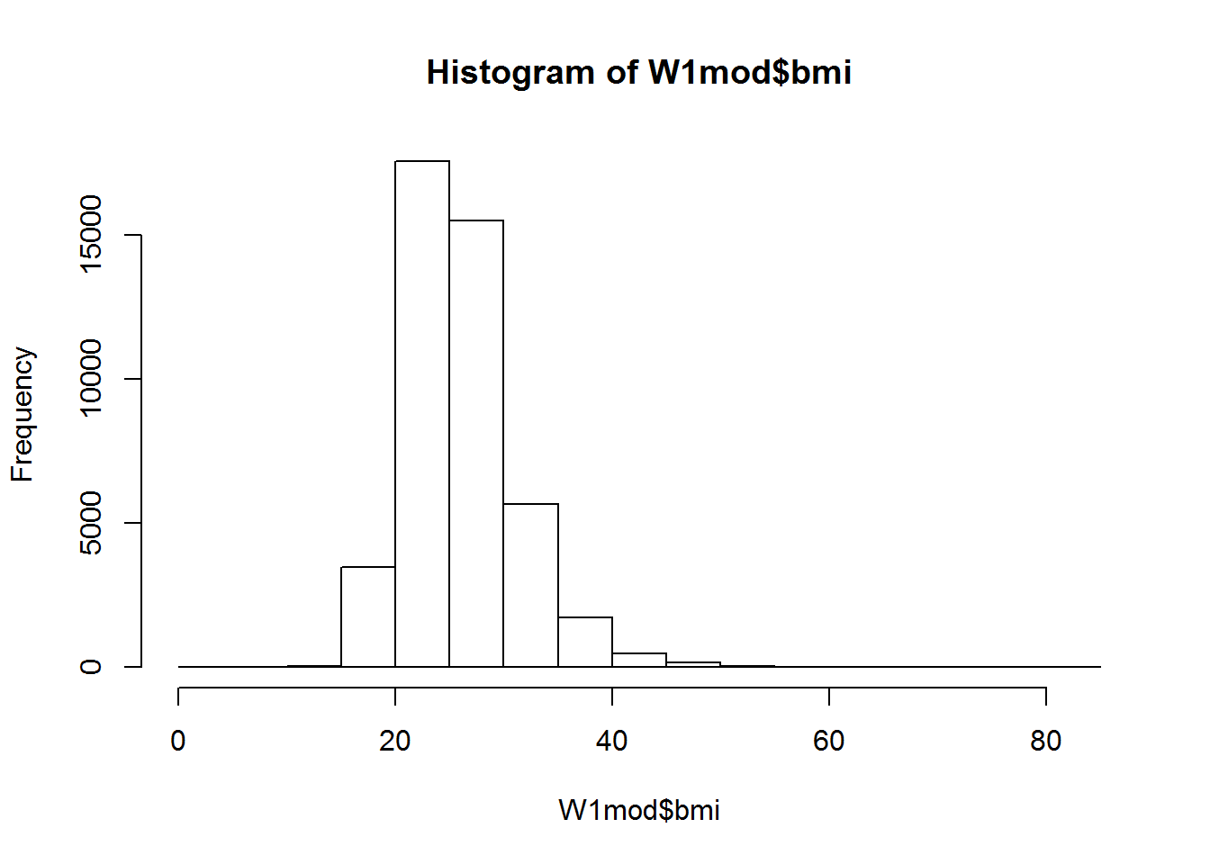
3.8 Sort data
We can sort data with the arrange() command from dplyr.
Initially, we sort the data by BMI.
W1mod %>%
  arrange(bmi) %>%
  select(pidp, bmi) %>%
  head(5)
## pidp bmi
## 1 614152207 3.581188
## 2 1158204567 4.357708
## 3 1292128539 10.098136
## 4 1088805127 11.732290
## 5 478722727 12.050592However, we can also sort data by a number of factors. Finally, we sort by BMI in decreasing order, separately for each sex.
library(tidyverse)
W1mod %>%
  arrange(a_sex, desc(bmi)) %>%
  select(pidp, a_sex, bmi) %>%
  head(5)
## pidp a_sex bmi
## 1 952435887 1 73.90269
## 2 1632274047 1 66.37745
## 3 340892847 1 65.19274
## 4 1292157767 1 63.10072
## 5 340443367 1 62.98222Here, we have just printed the first five rows of this data as an example. If you wanted, you could save these ordered datasets in the working environment, the same way we saved our new datasets earlier.